PMSM Parameter Identification in All-in-One-Servo Motors
Jia Li
Introduction
Permanent magnet synchronous machines (PMSMs) are prevalent in the industry due to their high efficiency, power density, and excellent mechanical dynamics. Field-oriented control (FOC) is normally used to drive PMSMs to improve their dynamic response and utilize the machine’s full potential. PMSM vector control contains a current loop, as well as mechanical, electrical, speed, and position loops. To achieve a control design with optimal performance, accurate and precise machine parameters are needed to build a proper mathematic model for the PMSM control system.
Datasheets are not always available, and even when they are, they often do not consider the operating conditions that each machine encounters. This article will address a method to identify parameters for PMSMs. A simple way to solve this dilemma is to use a motor control module. This motor’s algorithm should be based on the recursive least square (RLS) algorithm, with a forgetting factor that allows it to modify and monitor PMSM changes in real time.
Field-Oriented Control (FOC) in PMSMs
The basic idea of FOC is to be able to separately control the field flux and torque, similarly to how DC motors are controlled. Following the Clarke and Park transformations, a PMSM model under the synchronous rotating Q-D frame can be calculated using Equation (1), Equation (2), Equation (3), and Equation (4):
$$v_{QS}=r_S+ω_Rλ_{DS}+ρλ_{QS}$$$$v_{DS}=r_{S}-ω_rλ_{QS}+ρλ_{DS}$$
$$λ_{QS}=L_Si_{QS}+L_Mi_{QR}$$
$$λ_{DS}=L_Si_{DS}+L_M i_{DR}$$
Where the subscripts Q and D refer to the Q-axis and D-axis variables, respectively, LS is the machine’s self-inductance, and LM is the machine’s mutual inductance.
To further simplify the control, the rotor flux should be aligned on the D-axis while there is zero rotor flux on the Q-axis. The flux for the Q-axis and D-axis can be estimated with Equation (5) and Equation (6), respectively:
$$λ_{QS}=L_Si_{QS}$$$$λ_{DS}=L_Si_{DS}+λ_M^{'}$$
The electromagnetic torque can be calculated with Equation (7):
$$T_E= \frac {3} {2} \frac {P}{2} (λ'_{M}i_{QS} + (L_{D} - L_{Q}) i_{DS}i_{QS}) $$Following the transformation steps from the equations above, the magnetic flux can be directly controlled by the D-axis current. With a constant IDS, the torque (TE) can be directly controlled by manipulating the Q-axis current. If IDS = 0, then the electromagnetic torque is directly proportional to IQS.
The FOC of the PMSM schematic can be obtained using the derivations above (see Figure 1).
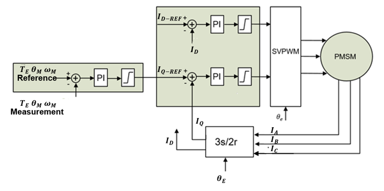
Figure 1: PMSM Vector Control
The outer loop reference can be the desired torque, machine speed, or certain shaft position. The outer loop reference is compared to the measured variables, and feeds the error to a controller (most commonly a PI controller) to generate the command torque current (IQ-REF).
The D-axis current reference (ID-REF) is set according to the magnetic flux requirement. The outputs of the current regulators/controllers (VQ-REF and VD-REF) are the input for the space vector PWM (SVPWM). The SVPWM block generates the gate signals for the inverter to drive the PMSM.
To achieve the desired dynamic performance of the PMSM servo machine, a motor control module can provide a controlled parameter with auto-tuning features. The motor control module can tune each PI controller automatically based on the given bandwidth requirements.
For current loop, the open-loop transfer function can be estimated with Equation (8):
$$G = \frac{KPS+K1} {S} \frac {1}{L_{S}S + r_S}$$Given a current bandwidth equals S = jω, the PMSM control parameters (KP and KI) can be back calculated based on the stator resistance and inductance.
Similar to the current loop, the outer loop (mechanical loop) open-loop function can be calculated with Equation (9):
$$G = \frac{KPS+K1} {S} \frac {kt}{JS + B}$$Where kt is the machine torque constant, J is the inertia, and B is the friction coefficient.
From Equation (9), the control parameter for outer loop can be calculated knowing the machine torque constant (kt), inertia (J), and friction coefficient (B).
Recursive Least Square Algorithm
The recursive least squares algorithm (RLS) is the recursive application of the least squares (LS) regression algorithm. New data is taken at each iteration to modify the system’s previous estimate.
The system output (y(t)) can be calculated with Equation (10):
$$y(t)=ϕ^T (t)θ(t)$$Where ϕ is the system input matrix, and θ is the PMSM system parameter.
Use $$\hatθ$$ to indicate the estimated system parameters. The objective function, or the term that is meant to be minimized or maximized, can be estimated with Equation (11):
$$J(θ,t)= \frac {1}{2} ∑_{i=1}^t(y(i)-\phi^T (i) \hatθ (i)) $$A new matrix for P and L can be calculated with Equation (12) and Equation (13), respectively:
$$P^{-1} (t)=∑_{i=1}^t\phi(i)\phi^T(i)$$ $$L(t)=P(t)\phi(t)$$The recursive least square parameter identification scheme is estimated with Equation (14), Equation (15), Equation (16), Equation (17), and Equation (18):
$$ϵ(t)=(y(t)-\phi^T (t)) \hatθ (t-1)$$$$L(t)=P(t-1)\phi(t) (I+\phi^T (t)P(t-1)\phi(t))^{-1}$$
$$P(t)=(I-L(t)\phi^T (t))P(t-1)$$
$$\hatθ(t)=\hatθ (t-1)+L(t)ϵ(t)$$
$$t=t+1$$
Adding a forgetting factor to the algorithm allows the scheme to handle a time-varying system. The weight given to the forgetting factor data depends on how old the data is, as the old data has less of an impact on the current iteration. The newest data is given the greatest weight for the algorithm. The forgetting factor (λ) ranges between [0,1]. The new objective function can be estimated with Equation (19):
$$J(θ,t)=\frac {1}{2} ∑_{i=1}^tλ^{t-i} (y(i)-\phi^T (i)\hat θ (i)) $$With the new objective function in Equation (19), the nth oldest data has a weight of λn. The recursive least square with a forgetting factor scheme can be calculated with Equation (20), Equation (21), Equation (22), Equation (23), and Equation (24):
$$ ϵ(t)=(y(t)-\phi^T (t)) \hatθ (t-1)$$$$L(t)=P(t-1)\phi(t) (λI+\phi^T (t)P(t-1)\phi(t))^{-1}$$
$$P(t)= \frac {1}{λ}(I-L(t) \phi^T (t))P(t-1)$$
$$\hatθ (t)=\hatθ (t-1)+L(t)ϵ(t)$$
$$t=t+1$$
Experimental Results
The MMS757188-36-R1-1 was used to validate the results. Table 1 lists the parameters from its datasheet.
Table 1: Motor Parameters
| Stator Phase Resistance | 300mΩ |
| Stator Phase Inductance | 350µH |
| Motor Inertia | 410gxcm2 |
| Torque Constant | 57mN x m/A |
| Pole Pairs | 4 |
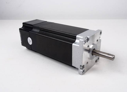
Figure 2: EZmotion Motor (MMS757188-36-R1-1)
Set the initial starting point to [0 0 0 0 0]T for the following motor parameters: phase resistance (RS), Q-axis inductance (LQ), D-axis inductance (LD), torque constant (kt), and motor shaft inertia (J).
For the RLS algorithm, the initial P matrix is set to P = 10000 x I5 x 5, and the forgetting factor is set to λ = 0.99.
Apply the starting conditions to the motor control module to perform the RLS motor parameter algorithm. Figure 3, Figure 4, Figure 5, Figure 6, and Figure 7 show the hardware experimental results.
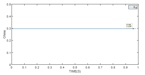
Figure 3: Experimental Results of Resistance Identification
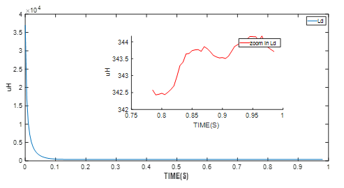
Figure 4: Experimental Results of D-Axis Resistance Identification
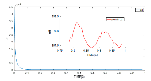
Figure 5: Experimental Results of Q-Axis Resistance Identification
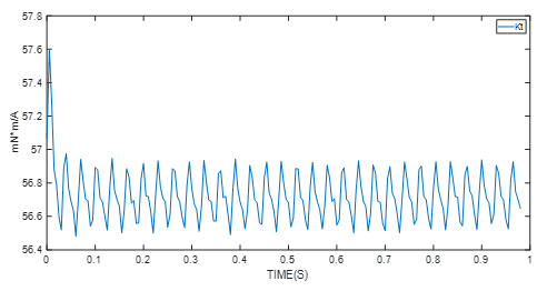
Figure 6: Experimental Results of Torque Constant Identification
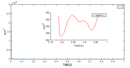
Figure 7: Experimental Results of Shaft Inertia Identification
The motor control module — the MMS757188-36-R1-1 in this example — detects whether the parameter identification algorithm has entered the stable phase. After the algorithm has entered the stable state shown in the graphs above, the final values are used. These values are the average motor parameter values.
Table 2: Identified Motor Parameters
| Stator Phase Resistance | 297mΩ |
| D-Axis Inductance | 343µH |
| Q-Axis Inductance | 358µH |
| Motor Inertia | 390gxcm2 |
| Torque Constant | 57mNxm/A |
| Pole Pairs | 4 |
Control Loop Auto-Tuning
As demonstrated in the previous section, the motor parameters impact the control parameters for the FOC of the PMSM. To help engineers achieve the desired motor performance, the control kit comes with a motor control module that auto-tunes the control parameters using the system transfer function developed in Equation (8) and Equation (9). If the motor parameters are available, the engineer only needs to input the desired bandwidth for each loop via the GUI. The host computer calculates the control parameters for the motor, then flashes the control parameter to the motor to ensure the performance.
PMSM control transfer functions are highly dependent on the motor parameters. If the motor parameters are incorrect, the motor does not perform effectively. This problem is explored further in the example below regarding changing the shaft inertia (J).
PMSMs are often utilized as high-performance servo motors. Their working conditions vary from case to case. The engineer may have an accurate motor parameter datasheet, or may have to measure the motor parameters by hand. Once the motor is placed in a complicated mechanical system, it is difficult to determine the shaft inertia.
The MMS757188-36-R1-1 can be used to drive a rotating disc (see Figure 8). The rotating disc increases the shaft inertia from 410gxcm2 to 7100gxcm2. The FOC is designed to have a position bandwidth of 20Hz, a speed bandwidth of 200Hz, and a current bandwidth of 2000Hz.
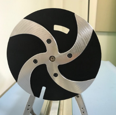
Figure 8: Motor Driving Spinning Disk
If the motor parameters used are taken from a device’s datasheet, the auto-tuning algorithm designs the control loop using the expected loop bandwidth, and the wrong motor parameter since the datasheet only offers the no-load inertia. The position reference is a ramp reference with a slope of 10rad/s. Figure 9 shows that when the position loop is out of control, the position feedback has a big oscillation.
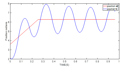
Figure 9: Position Control Performance with Original J Value
Using the motor control module, run the parameter identification algorithm. The motor parameter is updated to the current working conditions for the motor, and the auto-tuning algorithm helps the engineer tune the control loop based on the motor parameters under working conditions. The same position reference is used for the motor, and the position feedback tracks the reference with a stable error around 0.03% (see Figure 10).
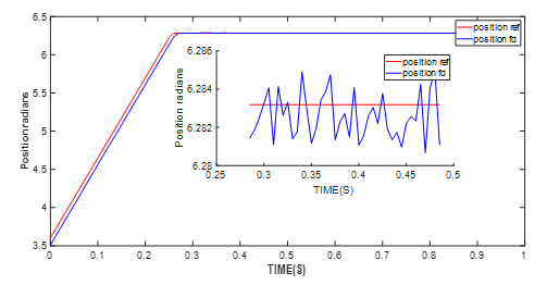
Figure 10: Position Control Performance with Updated J Value
Conclusion
This article presents solutions for RLS-based motor parameter identification for PMSMs using a motor control module. The performance is validated in hardware real-time tests using the MMS757188-36-R1-1. An example of position controls with different inertia values was presented to illustrate the significance of parameter identification. It was also demonstrated that other parameters have an impact on the control loop, since the PMSM FOC is dependent on multiple motor parameters.
Validate your login
Log in to your account
Create New Account